Vector-space models: designs, distances, basic reweighting

__author__ = "Christopher Potts"
__version__ = "CS224u, Stanford, Spring 2019"

# 이 문서는, 아파치 라이선스 2.0 하에, Christopher Potts 교수님의 CS224U 과목을 공부하면서 설명을 추가(번역 아님)한 자료 입니다.

Overview
Motivation
Terminological notes
Set-up
Matrix designs
Pre-computed example matrices
Vector comparison
Distributional neighbors
Matrix reweighting
Subword information
Visualization
Exploratory exercises

Overview

This notebook is the first in our series about creating effective distributed representations. The focus is on matrix designs, assessing similarity, and methods for matrix reweighting.

The central idea (which takes some getting used to!) is that we can represent words and phrases as dense vectors of real numbers. These take on meaning by being embedded in a larger matrix of representations with comparable structure.

matrix design, similarity 계산, matrix reweighting 등 distributed representation 에 대해 알아보겠습니다.

Motivation

Why build distributed representations? There are potentially many reasons. The two we will emphasize in this course:

Understanding words in context: There is value to linguists in seeing what these data-rich approaches can teach use about natural language lexicons, and there is value for social scientists in understanding how words are being used.
Feature representations for other models: As we will see, many models can benefit from representing examples as distributed representations.

(1) word를 context 상에서 이해할 수 있고, (2) 다른 어떤 모델의 feature representation으로 활용 가능하다는 점에 있어서, distributed representation을 build하는 것은 의미가 있습니다.

Terminological notes

The distributed representations we build will always be vectors of real numbers. The models are often called vector space models (VSMs).
Distributional representations are the special case where the data come entirely from co-occurrence counts in corpora.
We’ll look at models that use supervised labels to obtain vector-based word representations. These aren’t purely distributional, in that they take advantage of more than just co-occurrence patterns among items in the vocabulary, but they share the idea that words can be modeled with vectors.
If a neural network is used to train the representations, then they might be called neural representations.
The term word embedding is also used for distributed representations, including distributional ones. This term is a reminder that vector representations are meaningful only when embedded in and compared with others in a unified space (usually a matrix) of representations of the same type.
In any case, distributed representation seems like the most general cover term for what we’re trying to achieve, and its only downside is that sometimes people think it has something to do with distributed databases.
distributed representation을 build하면 실수 vector로 표현되며, 이 모델을 vector space model(VSM) 이라고도 부릅니다.
여러 코퍼스들에서 co-occurrence(동시발생) 카운트에서 전체적으로 데이터가 도출된 경우, distributional representation 이라고 합니다.
representation을 뉴럴넷을 활용해서 학습시킨 경우는, neural representation 이라고 합니다.
word embedding 은 distributed representation에 사용될 수도 있고, distributional representation에 사용될 수도 있다.
distributed representation 이 가장 일반적인 용어, 통칭할 수 있는 용어로 사용될 수 있음 (단, 분산DB와 아무 관련 없는 용어)

From Frequency to Meaning: Vector Space Models for Semantics 참고

Set-up

Make sure your environment meets all the requirements for the cs224u repository. For help getting set-up, see setup.ipynb.
Download the course data, unpack it, and place it in the directory containing the course repository – the same directory as this notebook. (If you want to put it somewhere else, change DATA_HOME below.)
vsm.py에 있는 구현체를, 이 노트북에 바로 입력해서 살펴볼 예정
imdb corpus가 yelp corpus로 변경되어 있음에 따라, 수정해서 실습 예정

%matplotlib inline
import numpy as np
import os
import pandas as pd
# import vsm
import scipy
import scipy.spatial.distance
from collections import defaultdict
import matplotlib.pyplot as plt
from sklearn.decomposition import PCA
from sklearn.manifold import TSNE

DATA_HOME = os.path.join('data', 'vsmdata')
!ls $DATA_HOME

giga_window20-flat.csv.gz  yelp_window20-flat.csv.gz
giga_window5-scaled.csv.gz yelp_window5-scaled.csv.gz

Matrix designs

There are many, many ways to define distributional matrices. Here’s a schematic overview that highlights the major decisions for building a word $\times$ word matrix:

Define a notion of co-occurrence context. This could be an entire document, a paragraph, a sentence, a clause, an NP — whatever domain seems likely to capture the associations you care about.
Define a count scaling method. The simplest method just counts everything in the context window, giving equal weight to everything inside it. A common alternative is to scale the weights based on proximity to the target word – e.g., $1/d$, where $d$ is the distance in tokens from the target.
Scan through your corpus building a dictionary $d$ mapping word-pairs to co-occurrence values. Every time a pair of words $w$ and $w’$ occurs in the same context (as you defined it in 1), increment $d[(w, w’)]$ by whatever value is determined by your weighting scheme. You’d increment by $1$ with the weighting scheme that simply counts co-occurrences.
Using the count dictionary $d$ that you collected in 3, establish your full vocabulary $V$, an ordered list of words types.
1. For large collections of documents, $|V|$ will typically be huge. You will probably want to winnow the vocabulary at this point.
2. You might do this by filtering to a specific subset, or just imposing a minimum count threshold.
3. You might impose a minimum count threshold even if $|V|$ is small — for words with very low counts, you simply don’t have enough evidence to support good representations.
4. For words outside the vocabulary you choose, you could ignore them entirely or accumulate all their values into a designated UNK vector.
Now build a matrix $M$ of dimension $|V| \times |V|$. Both the rows and the columns of $M$ represent words. Each cell $M[i, j]$ is filled with the value $d[(w_{i}, w_{j})]$.

distributional matrix를 정의하는데 많은 방법이 있지만, word $\times$ word matrix를 build하는 데 아래 순서로 가능:

co-occurrence context 의 개념을 정의할 것. 전체 문서, 단락, 문장, 절, 명사구(Noun Phrase) 등 연관관계를 보려는 어떤 것이라도 될 수 있음.
카운트 스케일링 메소드 를 정의할 것. context window 내의 모든 토큰에 같은 weight을 주는 가장 간단한 방법도 있고, 타겟 토큰으로 부터 얼마나 떨어졌는지 거리($d$)에 따라 $1/d$로 weight를 scaling할 수도 있음.
코퍼스를 스캔해서 단어쌍에 co-occurrence 값을 매핑하는 사전 $d$를 build할 것. 1번에서 정의했던 같은 context 내에서 등장한 단어 $w$와 $w’$의 쌍 마다, 2번에서 정의한 weighting shceme으로 값을 증가시키기.
3번에 서 만든 카운트 사전 $d$를 이용해서 전체 vocab $V$ (word type의 ordered list)를 만들기.
행과 열이 word인 $|V| \times |V|$인 행렬 $M$ 만들기. $M[i,j]$의 각 셀은 단어쌍 거리의 값($d[(w_{i}. w_{j})]$)으로 채워져있음.

Pre-computed example matrices

The data distribution includes four matrices that we’ll use for hands-on exploration. All of them were designed in the same basic way:

They are word $\times$ word matrices with 6K rows and 6K columns.
The vocabulary is the top 6K most frequent unigrams.

Two come from Yelp user-supplied reviews, and two come from Gigaword, a collection of newswire and newspaper text. Further details:

filename	source	window size	count weighting
yelp_window5-scaled.csv.gz	Yelp reviews	5	1/d
yelp_window20-flat.csv.gz	Yelp reviews	20	1
gigaword_window5-scaled.csv.gz	Gigaword	5	1/d
gigaword_window20-flat.csv.gz	Gigaword	20	1

Any hunches about how these matrices might differ from each other?

yelp5 = pd.read_csv(
    os.path.join(DATA_HOME, 'yelp_window5-scaled.csv.gz'), index_col=0)
yelp5

	):	);	..	...	:(	:)	:/	:D	:\|	;p	...	younger	your	yourself	youth	zebra	zero	zinc	zombie	zone	zoo
):	154.566667	0.000000	16.516667	60.750000	2.550000	8.466667	0.000000	0.866667	0.000000	0.00	...	0.666667	40.516667	4.616667	0.416667	0.000000	4.450000	0.000000	0.166667	0.166667	0.333333
);	0.000000	24.866667	3.200000	36.200000	0.000000	1.000000	0.000000	0.000000	0.000000	0.00	...	0.250000	32.733333	2.200000	0.000000	0.000000	0.533333	0.000000	0.250000	0.450000	0.700000
..	16.516667	3.200000	13494.866667	6945.366667	196.750000	501.650000	40.450000	29.400000	0.700000	2.15	...	31.850000	2908.116667	247.366667	3.183333	1.783333	146.733333	1.250000	9.733333	23.816667	20.300000
...	60.750000	36.200000	6945.366667	62753.766667	783.216667	1711.583333	161.383333	101.700000	4.883333	7.85	...	119.100000	12530.533333	1259.683333	29.550000	4.516667	675.816667	8.833333	33.400000	108.783333	77.583333
:(	2.550000	0.000000	196.750000	783.216667	423.433333	13.950000	2.133333	0.166667	0.366667	0.00	...	0.333333	72.433333	5.333333	0.000000	0.000000	7.650000	0.000000	0.533333	4.533333	0.166667
...	...	...	...	...	...	...	...	...	...	...	...	...	...	...	...	...	...	...	...	...	...
zero	4.450000	0.533333	146.733333	675.816667	7.650000	8.183333	0.750000	0.200000	0.000000	0.00	...	1.466667	121.233333	11.483333	0.333333	0.000000	476.733333	0.000000	0.783333	3.583333	0.866667
zinc	0.000000	0.000000	1.250000	8.833333	0.000000	0.500000	0.000000	0.000000	0.000000	0.00	...	0.000000	2.600000	0.166667	0.000000	0.000000	0.000000	2.066667	0.000000	0.000000	0.000000
zombie	0.166667	0.250000	9.733333	33.400000	0.533333	1.733333	0.000000	0.000000	0.000000	0.00	...	0.750000	20.700000	1.866667	0.000000	0.166667	0.783333	0.000000	25.400000	4.616667	0.500000
zone	0.166667	0.450000	23.816667	108.783333	4.533333	7.066667	0.000000	0.000000	0.000000	0.00	...	0.916667	257.866667	4.783333	0.000000	0.000000	3.583333	0.000000	4.616667	28.800000	0.000000
zoo	0.333333	0.700000	20.300000	77.583333	0.166667	4.850000	0.000000	0.000000	0.000000	0.00	...	1.000000	31.783333	3.533333	0.000000	0.333333	0.866667	0.000000	0.500000	0.000000	85.166667

6000 rows × 6000 columns

yelp20 = pd.read_csv(
    os.path.join(DATA_HOME, 'yelp_window20-flat.csv.gz'), index_col=0)
yelp20

	):	);	..	...	:(	:)	:/	:D	:\|	;p	...	younger	your	yourself	youth	zebra	zero	zinc	zombie	zone	zoo
):	3910.0	24.0	250.0	1162.0	48.0	261.0	4.0	22.0	0.0	1.0	...	6.0	945.0	61.0	3.0	1.0	27.0	1.0	1.0	2.0	3.0
);	24.0	1738.0	55.0	595.0	7.0	27.0	0.0	2.0	0.0	0.0	...	5.0	564.0	29.0	0.0	0.0	7.0	0.0	2.0	3.0	5.0
..	250.0	55.0	330680.0	154726.0	1605.0	5707.0	311.0	336.0	10.0	21.0	...	437.0	40631.0	2680.0	36.0	12.0	1441.0	8.0	107.0	237.0	182.0
...	1162.0	595.0	154726.0	1213778.0	6404.0	21831.0	1230.0	1172.0	41.0	73.0	...	1684.0	174619.0	13862.0	323.0	57.0	6345.0	71.0	405.0	1208.0	840.0
:(	48.0	7.0	1605.0	6404.0	1646.0	528.0	55.0	33.0	4.0	1.0	...	9.0	1425.0	84.0	1.0	1.0	66.0	0.0	5.0	15.0	7.0
...	...	...	...	...	...	...	...	...	...	...	...	...	...	...	...	...	...	...	...	...	...
zero	27.0	7.0	1441.0	6345.0	66.0	110.0	6.0	4.0	0.0	0.0	...	43.0	4141.0	368.0	4.0	0.0	3894.0	0.0	14.0	28.0	19.0
zinc	1.0	0.0	8.0	71.0	0.0	4.0	0.0	0.0	0.0	0.0	...	0.0	34.0	7.0	0.0	0.0	0.0	98.0	0.0	0.0	0.0
zombie	1.0	2.0	107.0	405.0	5.0	22.0	0.0	4.0	0.0	0.0	...	3.0	287.0	28.0	1.0	1.0	14.0	0.0	604.0	22.0	1.0
zone	2.0	3.0	237.0	1208.0	15.0	62.0	1.0	1.0	0.0	0.0	...	14.0	1721.0	99.0	3.0	1.0	28.0	0.0	22.0	764.0	14.0
zoo	3.0	5.0	182.0	840.0	7.0	47.0	0.0	1.0	0.0	0.0	...	16.0	699.0	53.0	2.0	10.0	19.0	0.0	1.0	14.0	3148.0

6000 rows × 6000 columns

giga5 = pd.read_csv(
    os.path.join(DATA_HOME, 'giga_window5-scaled.csv.gz'), index_col=0)
giga5

	):	);	..	...	:(	:)	:/	:D	:\|	;p	...	younger	your	yourself	youth	zebra	zero	zinc	zombie	zone	zoo
):	4.300000	8.100000	7.700000	113.766667	2.666667	1.116667	0.50	0.0	0.0	0.0	...	2.850000	147.633333	8.483333	4.500000	0.000000	2.733333	0.200000	0.333333	344.066667	0.700000
);	8.100000	1092.400000	0.650000	52.783333	0.666667	0.000000	0.00	0.0	0.0	0.0	...	7.100000	44.400000	3.333333	7.116667	0.400000	1.616667	1.000000	0.500000	11.516667	1.250000
..	7.700000	0.650000	18900.766667	12657.800000	0.500000	0.500000	0.00	0.5	0.0	0.0	...	1.166667	29.883333	0.833333	0.250000	0.000000	0.916667	0.250000	0.000000	2.983333	1.083333
...	113.766667	52.783333	12657.800000	131656.033333	0.866667	0.500000	0.85	0.0	0.0	0.0	...	40.333333	2187.066667	89.750000	42.000000	8.200000	30.683333	0.666667	2.333333	79.233333	11.083333
:(	2.666667	0.666667	0.500000	0.866667	0.000000	0.333333	0.00	0.0	0.0	0.0	...	0.000000	0.333333	0.000000	0.666667	0.000000	0.000000	0.000000	0.000000	0.000000	0.000000
...	...	...	...	...	...	...	...	...	...	...	...	...	...	...	...	...	...	...	...	...	...
zero	2.733333	1.616667	0.916667	30.683333	0.000000	0.000000	0.00	0.0	0.0	0.0	...	0.666667	26.516667	1.533333	1.600000	0.000000	270.333333	0.000000	0.000000	6.900000	0.000000
zinc	0.200000	1.000000	0.250000	0.666667	0.000000	0.000000	0.00	0.0	0.0	0.0	...	0.000000	7.116667	0.000000	0.000000	0.000000	0.000000	24.966667	0.000000	0.000000	0.000000
zombie	0.333333	0.500000	0.000000	2.333333	0.000000	0.000000	0.00	0.0	0.0	0.0	...	0.200000	2.700000	0.000000	0.250000	0.000000	0.000000	0.000000	4.700000	0.500000	0.000000
zone	344.066667	11.516667	2.983333	79.233333	0.000000	0.000000	0.00	0.0	0.0	0.0	...	1.000000	112.033333	3.850000	2.333333	0.666667	6.900000	0.000000	0.500000	248.466667	0.816667
zoo	0.700000	1.250000	1.083333	11.083333	0.000000	0.000000	0.25	0.0	0.0	0.0	...	1.000000	9.383333	0.250000	0.400000	1.500000	0.000000	0.000000	0.000000	0.816667	141.133333

6000 rows × 6000 columns

giga20 = pd.read_csv(
    os.path.join(DATA_HOME, 'giga_window20-flat.csv.gz'), index_col=0)
giga20

	):	);	..	...	:(	:)	:/	:D	:\|	;p	...	younger	your	yourself	youth	zebra	zero	zinc	zombie	zone	zoo
):	7046.0	517.0	29.0	1684.0	45.0	10.0	15.0	0.0	1.0	0.0	...	34.0	2716.0	318.0	75.0	0.0	18.0	11.0	5.0	1128.0	11.0
);	517.0	108712.0	19.0	288.0	15.0	0.0	0.0	1.0	1.0	0.0	...	105.0	872.0	34.0	80.0	5.0	19.0	15.0	5.0	111.0	13.0
..	29.0	19.0	101566.0	116373.0	1.0	1.0	6.0	2.0	0.0	0.0	...	72.0	886.0	17.0	24.0	23.0	75.0	33.0	0.0	225.0	10.0
...	1684.0	288.0	116373.0	1627084.0	27.0	48.0	7.0	3.0	0.0	0.0	...	671.0	27690.0	1158.0	886.0	392.0	417.0	6.0	34.0	1522.0	149.0
:(	45.0	15.0	1.0	27.0	50.0	5.0	2.0	1.0	0.0	0.0	...	1.0	49.0	3.0	2.0	0.0	0.0	0.0	0.0	1.0	0.0
...	...	...	...	...	...	...	...	...	...	...	...	...	...	...	...	...	...	...	...	...	...
zero	18.0	19.0	75.0	417.0	0.0	0.0	0.0	0.0	0.0	0.0	...	25.0	596.0	49.0	26.0	0.0	3460.0	2.0	0.0	140.0	7.0
zinc	11.0	15.0	33.0	6.0	0.0	0.0	0.0	0.0	3.0	0.0	...	0.0	85.0	2.0	1.0	0.0	2.0	1366.0	0.0	2.0	1.0
zombie	5.0	5.0	0.0	34.0	0.0	0.0	0.0	0.0	0.0	0.0	...	3.0	65.0	1.0	3.0	0.0	0.0	0.0	188.0	3.0	0.0
zone	1128.0	111.0	225.0	1522.0	1.0	0.0	0.0	1.0	0.0	1.0	...	54.0	1464.0	60.0	52.0	7.0	140.0	2.0	3.0	11250.0	19.0
zoo	11.0	13.0	10.0	149.0	0.0	0.0	1.0	0.0	0.0	0.0	...	34.0	257.0	15.0	16.0	36.0	7.0	1.0	0.0	19.0	5568.0

6000 rows × 6000 columns

Vector comparison

Vector comparisons form the heart of our analyses in this context.

For the most part, we are interested in measuring the distance between vectors. The guiding idea is that semantically related words should be close together in the vector spaces we build, and semantically unrelated words should be far apart.
The scipy.spatial.distance module has a lot of vector comparison methods, so you might check them out if you want to go beyond the functions defined and explored here. Read the documentation closely, though: many of those methods are defined only for binary vectors, whereas the VSMs we’ll use allow all float values.

Euclidean

The most basic and intuitive distance measure between vectors is euclidean distance. The euclidean distance between two vectors $u$ and $v$ of dimension $n$ is

\[\textbf{euclidean}(u, v) = \sqrt{\sum_{i=1}^{n}|u_{i} - v_{i}|^{2}}\]

In two-dimensions, this corresponds to the length of the most direct line between the two points.

In vsm.py, the function euclidean just uses the corresponding scipy.spatial.distance method to define it.

Here’s the tiny vector space from the screencast on vector comparisons associated with this notebook:

Running example
• Focus on distance measures
• Illustrations with row vectors
어떤 문서(혹은 코퍼스 등) x, y에, A, B, C라는 단어가 등장한다고 할 때
혹은, 어떤 단어 x, y와, A, B, C라는 단어가 함께 등장한다고 할 때

ABC = pd.DataFrame([
    [ 2.0,  4.0], 
    [10.0, 15.0], 
    [14.0, 10.0]],
    index=['A', 'B', 'C'],
    columns=['x', 'y'])

ABC

	x	y
A	2.0	4.0
B	10.0	15.0
C	14.0	10.0

def plot_ABC(df):
    ax = df.plot.scatter(x='x', y='y', marker='.', legend=False)
    m = df.values.max(axis=None)
    ax.set_xlim([0, m*1.2])
    ax.set_ylim([0, m*1.2])
    for label, row in df.iterrows():
        ax.text(row['x'], row['y'], label)

plot_ABC(ABC)

png

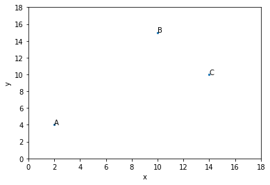
The euclidean distances align well with raw visual distance in the plot:

def euclidean(u, v):
    return scipy.spatial.distance.euclidean(u, v)

def abc_comparisons(df, distfunc):
    """(A,B)간, (B,C)간 거리 함수를 parameter로 받아서, 두 점 사이의 거리를 계산하는 함수
    """
    for a, b in (('A', 'B'), ('B', 'C')):
        dist = distfunc(df.loc[a], df.loc[b]) # df.loc[a]: Series type
        print('{0:}({1:}, {2:}) = {3:7.02f}'.format(
            distfunc.__name__, a, b, dist))

abc_comparisons(ABC, euclidean) # plain X, Y축 값을 갖는 dataframe ABC를 넘김.

euclidean(A, B) =   13.60
euclidean(B, C) =    6.40

However, suppose we think of the vectors as word meanings in the vector-space sense. In that case, the values don’t look good:

The distributions of B and C are more or less directly opposed, suggesting very different meanings, whereas A and B are rather closely aligned, abstracting away from the fact that the first is far less frequent than the second.
In terms of the large models we will soon explore, A and B resemble a pair like superb and good, which have similar meanings but very different frequencies.
In contrast, B and C are like good and disappointing — similar overall frequencies but different distributions with respect to the overall vocabulary.

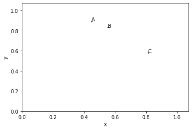
Length normalization

These affinities are immediately apparent if we normalize the vectors by their length. To do this, we first define the L2-length of a vector:

\[\|u\|_{2} = \sqrt{\sum_{i=1}^{n} u_{i}^{2}}\]

And then the normalization step just divides each value by this quantity:

\[\left[ \frac{u_{1}}{\|u\|_{2}}, \frac{u_{2}}{\|u\|_{2}}, \ldots \frac{u_{n}}{\|u\|_{2}} \right]\]

def vector_length(u):
    """
    u vector의 dot(inner) product 
    ([1, 2, 3]).dot([1, 2, 3]) = 1+4+9 = 14
    """
    return np.sqrt(u.dot(u)) 

def length_norm(u):
    return u / vector_length(u)

ABC_normed = ABC.apply(length_norm, axis=1)

plot_ABC(ABC_normed)

png

abc_comparisons(ABC_normed, euclidean) # normalize된 ABC dataframe의 euclidean distance

euclidean(A, B) =    0.12
euclidean(B, C) =    0.36

Here, the connection between A and B is more apparent, as is the opposition between B and C.

Cosine distance

Cosine distance takes overall length into account. The cosine distance between two vectors $u$ and $v$ of dimension $n$ is

\[\textbf{cosine}(u, v) = 1 - \frac{\sum_{i=1}^{n} u_{i} \cdot v_{i}}{\|u\|_{2} \cdot \|v\|_{2}}\]

The similarity part of this (the righthand term of the subtraction) is actually measuring the angles between the two vectors. The result is the same (in terms of rank order) as one gets from first normalizing both vectors using $|\cdot|_{2}$ and then calculating their Euclidean distance.

def cosine(u, v):
    return scipy.spatial.distance.cosine(u, v)

abc_comparisons(ABC, cosine)

cosine(A, B) =    0.01
cosine(B, C) =    0.07

So, in building in the length normalization, cosine distance achieves our goal of associating A and B and separating both from C.

Matching-based methods

Matching-based methods are also common in the literature. The basic matching measure effectively creates a vector consisting of all of the smaller of the two values at each coordinate, and then sums them:

\[\textbf{matching}(u, v) = \sum_{i=1}^{n} \min(u_{i}, v_{i})\]

This is implemented in vsm as matching.

One approach to normalizing the matching values is the Jaccard coefficient. The numerator is the matching coefficient. The denominator — the normalizer — is intuitively like the set union: for binary vectors, it gives the cardinality of the union of the two being compared:

\[\textbf{jaccard}(u, v) = 1 - \frac{\textbf{matching}(u, v)}{\sum_{i=1}^{n} \max(u_{i}, v_{i})}\]

Summary

Suppose we set for ourselves the goal of associating A with B and disassociating B from C, in keeping with the semantic intuition expressed above. Then we can assess distance measures by whether they achieve this goal:

def matching(u, v):
    return np.sum(np.minimum(u, v))

def jaccard(u, v):
    return 1.0 - (matching(u, v) / np.sum(np.maximum(u, v)))

for m in (euclidean, cosine, jaccard):
    fmt = {
        'n': m.__name__,  
        'AB': m(ABC.loc['A'], ABC.loc['B']), 
        'BC': m(ABC.loc['B'], ABC.loc['C'])}
    print('{n:>15}(A, B) = {AB:5.2f} {n:>15}(B, C) = {BC:5.2f}'.format(**fmt))

      euclidean(A, B) = 13.60       euclidean(B, C) =  6.40
         cosine(A, B) =  0.01          cosine(B, C) =  0.07
        jaccard(A, B) =  0.76         jaccard(B, C) =  0.31

Distributional neighbors

The neighbors function in vsm is an investigative aide. For a given word w, it ranks all the words in the vocabulary according to their distance from w, as measured by distfunc (default: vsm.cosine).

By playing around with this function, you can start to get a sense for how the distance functions differ. Here are some example uses; you might try some new words to get a feel for what these matrices are like and how different words look.

def neighbors(word, df, distfunc=cosine):
    """Tool for finding the nearest neighbors of `word` in `df` according
    to `distfunc`. The comparisons are between row vectors.

    Parameters
    ----------
    word : str
        The anchor word. Assumed to be in `rownames`.
    df : pd.DataFrame
        The vector-space model.
    distfunc : function mapping vector pairs to floats (default: `cosine`)
        The measure of distance between vectors. Can also be `euclidean`,
        `matching`, `jaccard`, as well as any other distance measure
        between 1d vectors.

    Raises
    ------
    ValueError
        If word is not in `df.index`.

    Returns
    -------
    pd.Series
        Ordered by closeness to `word`.

    """
    if word not in df.index:
        raise ValueError('{} is not in this VSM'.format(word))
    w = df.loc[word]
    dists = df.apply(lambda x: distfunc(w, x), axis=1)
    return dists.sort_values()

neighbors('A', ABC, distfunc=euclidean)

A     0.000000
C    13.416408
B    13.601471
dtype: float64

neighbors('A', ABC, distfunc=cosine)

A    0.000000
B    0.007722
C    0.116212
dtype: float64

neighbors('good', yelp5, distfunc=euclidean).head()

good          0.000000
great    363501.370559
very     463140.024533
there    484997.266143
so       503078.898630
dtype: float64

neighbors('good', yelp20, distfunc=euclidean).head()

good     0.000000e+00
very     1.582079e+06
food     1.706024e+06
as       2.180615e+06
great    2.309515e+06
dtype: float64

neighbors('good', yelp5, distfunc=cosine).head()

good          0.000000
decent        0.052814
weak          0.061491
impressive    0.063750
solid         0.072259
dtype: float64

neighbors('good', yelp20, distfunc=cosine).head()

good      0.000000
decent    0.005797
pretty    0.006568
really    0.007324
quite     0.007358
dtype: float64

neighbors('good', giga5, distfunc=euclidean).head()

good            0.000000
very        96629.020074
another    102967.358766
little     111678.083808
big        112087.562461
dtype: float64

neighbors('good', giga20, distfunc=euclidean).head()

good          0.000000
very     342311.566423
here     510760.069407
think    529750.740523
right    561272.646841
dtype: float64

neighbors('good', giga5, distfunc=cosine).head()

good       0.000000
bad        0.047839
painful    0.070546
simple     0.073625
safe       0.076624
dtype: float64

neighbors('good', giga20, distfunc=cosine).head()

good        0.000000
bad         0.004829
everyone    0.006463
always      0.006505
very        0.007011
dtype: float64

Matrix reweighting

The goal of reweighting is to amplify the important, trustworthy, and unusual, while deemphasizing the mundane and the quirky.
Absent a defined objective function, this will remain fuzzy, but the intuition behind moving away from raw counts is that frequency is a poor proxy for our target semantic ideas.

Normalization

Normalization (row-wise or column-wise) is perhaps the simplest form of reweighting. With vsm.length_norm, we normalize using vsm.vector_length. We can also normalize each row by the sum of its values, which turns each row into a probability distribution over the columns:

\[\left[ \frac{u_{1}}{\sum_{i=1}^{n}u_{i}}, \frac{u_{2}}{\sum_{i=1}^{n}u_{i}}, \ldots \frac{u_{n}}{\sum_{i=1}^{n}u_{i}}, \right]\]

These normalization measures are insensitive to the magnitude of the underlying counts. This is often a mistake in the messy world of large data sets; $[1,10]$ and $[1000,10000]$ are very different vectors in ways that will be partly or totally obscured by normalization.

Observed/Expected

Reweighting by observed-over-expected values captures one of the central patterns in all of VSMs: we can adjust the actual cell value in a co-occurrence matrix using information from the corresponding row and column.

In the case of observed-over-expected, the rows and columns define our expectation about what the cell value would be if the two co-occurring words were independent. In dividing the observed count by this value, we amplify cells whose values are larger than we would expect.

So that this doesn’t look more complex than it is, for an $m \times n$ matrix $X$, define

\[\textbf{rowsum}(X, i) = \sum_{j=1}^{n}X_{ij}\] \[\textbf{colsum}(X, j) = \sum_{i=1}^{m}X_{ij}\] \[\textbf{sum}(X) = \sum_{i=1}^{m}\sum_{j=1}^{n} X_{ij}\] \[\textbf{expected}(X, i, j) = \frac{ \textbf{rowsum}(X, i) \cdot \textbf{colsum}(X, j) }{ \textbf{sum}(X) }\]

Then the observed-over-expected value is

\[\textbf{oe}(X, i, j) = \frac{X_{ij}}{\textbf{expected}(X, i, j)}\]

In many contexts, it is more intuitive to first normalize the count matrix into a joint probability table and then think of $\textbf{rowsum}$ and $\textbf{colsum}$ as probabilities. Then it is clear that we are comparing the observed joint probability with what we would expect it to be under a null hypothesis of independence. These normalizations do not affect the final results, though.

Let’s do a quick worked-out example. Suppose we have the count matrix $X$ =

	a	b	rowsum
x	34	11	45
y	47	7	54
colsum	81	18	99

Then we calculate like this:

\[\textbf{oe}(X, 1, 0) = \frac{47}{\frac{54 \cdot 81}{99}} = 1.06\]

And the full table looks like this:

	a	b
x	0.92	1.34
y	1.06	0.71

def observed_over_expected(df):
    col_totals = df.sum(axis=0)
    total = col_totals.sum()
    row_totals = df.sum(axis=1)
    expected = np.outer(row_totals, col_totals) / total
    oe = df / expected
    return oe

oe_ex = np.array([[ 34.,  11.], [ 47.,   7.]])

observed_over_expected(oe_ex).round(2)

array([[0.92, 1.34],
       [1.06, 0.71]])

The implementation vsm.observed_over_expected should be pretty efficient.

yelp5_oe = observed_over_expected(yelp5)

yelp20_oe = observed_over_expected(yelp20)

neighbors('good', yelp5_oe).head()

good         0.000000
great        0.323037
decent       0.381849
but          0.403750
excellent    0.411684
dtype: float64

neighbors('good', yelp20_oe).head()

good      0.000000
too       0.058905
really    0.060264
pretty    0.064466
but       0.066778
dtype: float64

giga5_oe = observed_over_expected(giga5)

giga20_oe = observed_over_expected(giga20)

neighbors('good', giga5_oe).head()

good      0.000000
bad       0.485495
better    0.533762
well      0.553319
but       0.556113
dtype: float64

neighbors('good', giga20_oe).head()

good      0.000000
just      0.102044
so        0.106773
that's    0.108614
better    0.111044
dtype: float64

Pointwise Mutual Information

Pointwise Mutual Information (PMI) is observed-over-expected in log-space:

\[\textbf{pmi}(X, i, j) = \log\left(\frac{X_{ij}}{\textbf{expected}(X, i, j)}\right)\]

This basic definition runs into a problem for $0$ count cells. The usual response is to set $\log(0) = 0$, but this is arguably confusing – cell counts that are smaller than expected get negative values, cell counts that are larger than expected get positive values, and 0-count values are placed in the middle of this ranking without real justification.

For this reason, it is more typical to use Positive PMI, which maps all negative PMI values to $0$:

\[\textbf{ppmi}(X, i, j) = \begin{cases} \textbf{pmi}(X, i, j) & \textrm{if } \textbf{pmi}(X, i, j) > 0 \\ 0 & \textrm{otherwise} \end{cases}\]

This is the default for vsm.pmi.

def pmi(df, positive=True):
    df = observed_over_expected(df)
    # Silence distracting warnings about log(0):
    with np.errstate(divide='ignore'):
        df = np.log(df)
    df[np.isinf(df)] = 0.0  # log(0) = 0
    if positive:
        df[df < 0] = 0.0
    return df

yelp5_pmi = pmi(yelp5)

yelp20_pmi = pmi(yelp20)

neighbors('good', yelp5_pmi).head()

good         0.000000
decent       0.448116
great        0.466581
tasty        0.532094
excellent    0.569720
dtype: float64

neighbors('good', yelp20_pmi).head()

good         0.000000
tasty        0.201911
delicious    0.261547
flavorful    0.317310
ordered      0.349519
dtype: float64

giga5_pmi = pmi(giga5)

giga20_pmi = pmi(giga20)

neighbors('good', giga5_pmi).head()

good        0.000000
bad         0.439959
better      0.494448
terrific    0.509023
decent      0.520705
dtype: float64

neighbors('good', giga20_pmi).head()

good      0.000000
really    0.271877
that's    0.272447
it's      0.285056
pretty    0.294105
dtype: float64

neighbors('market', giga5_pmi).head()

market     0.000000
markets    0.327014
stocks     0.512569
prices     0.516767
sales      0.552022
dtype: float64

neighbors('market', giga20_pmi).head()

market     0.000000
markets    0.175934
prices     0.252851
stocks     0.266186
profits    0.269412
dtype: float64

TF-IDF

Perhaps the best known reweighting schemes is Term Frequency–Inverse Document Frequency (TF-IDF), which is, I believe, still the backbone of today’s Web search technologies. As the name suggests, it is built from TF and IDF measures:

For an $m \times n$ matrix $X$:

\[\textbf{TF}(X, i, j) = \frac{X_{ij}}{\textbf{colsum}(X, i, j)}\] \[\textbf{IDF}(X, i, j) = \log\left(\frac{n}{|\{k : X_{ik} > 0\}|}\right)\] \[\textbf{TF-IDF}(X, i, j) = \textbf{TF}(X, i, j) \cdot \textbf{IDF}(X, i, j)\]

TF-IDF generally performs best with sparse matrices. It severely punishes words that appear in many documents; if a word appears in every document, then its IDF value is 0. As a result, it can even be problematic with verb dense word $\times$ word matrices like ours, where most words appear with most other words.

There is an implementation of TF-IDF for dense matrices in vsm.tfidf.

Important: sklearn’s version, TfidfTransformer, assumes that term frequency (TF) is defined row-wise and document frequency is defined column-wise. That is, it assumes sklearn’s document $\times$ word basic design, which makes sense for classification tasks, where the design is example $\times$ features. This is the transpose of the way we’ve been thinking.

def tfidf(df):
    # Inverse document frequencies:
    doccount = float(df.shape[1])
    freqs = df.astype(bool).sum(axis=1)
    idfs = np.log(doccount / freqs)
    idfs[np.isinf(idfs)] = 0.0  # log(0) = 0
    # Term frequencies:
    col_totals = df.sum(axis=0)
    tfs = df / col_totals
    return (tfs.T * idfs).T

Subword information

Schütze (1993) pioneered the use of subword information to improve representations by reducing sparsity, thereby increasing the density of connections in a VSM. In recent years, this idea has shown value in numerous contexts.

Bojanowski et al. (2016) (the fastText team) explore a particularly straightforward approach to doing this: represent each word as the sum of the representations for the character-level n-grams it contains.

It is simple to derive character-level n-gram representations from our existing VSMs. The function vsm.ngram_vsm implements the basic step. Here, we create the 4-gram version of imdb5:

def ngram_vsm(df, n=2):
    """Create a character-level VSM from `df`.

    Parameters
    ----------
    df : pd.DataFrame
    n : int
        The n-gram size.

    Returns
    -------
    pd.DataFrame
        This will have the same column dimensionality as `df`, but the
        rows will be expanded with representations giving the sum of
        all the original rows in `df` that contain that row's n-gram.

    """
    unigram2vecs = defaultdict(list)
    for w, x in df.iterrows():
        for c in get_character_ngrams(w, n):
            unigram2vecs[c].append(x)
    unigram2vecs = {c: np.array(x).sum(axis=0)
                    for c, x in unigram2vecs.items()}
    cf = pd.DataFrame(unigram2vecs).T
    cf.columns = df.columns
    return cf

def get_character_ngrams(w, n):
    """Map a word to its character-level n-grams, with boundary
    symbols '<w>' and '</w>'.

    Parameters
    ----------
    w : str
    n : int
        The n-gram size.

    Returns
    -------
    list of str

    """
    if n > 1:
        w = ["<w>"] + list(w) + ["</w>"]
    else:
        w = list(w)
    return ["".join(w[i: i+n]) for i in range(len(w)-n+1)]

yelp5_ngrams = ngram_vsm(yelp5, n=4)

yelp5_ngrams.shape

(10382, 6000)

This has the same column dimension as the yelp5, but the rows are expanded with all the 4-grams, including boundary symbols <w> and </w>. Here’s a simple function for creating new word representations from the associated character-level ones:

def character_level_rep(word, cf, n=4):
    ngrams = get_character_ngrams(word, n)
    ngrams = [n for n in ngrams if n in cf.index]    
    reps = cf.loc[ngrams].values
    return reps.sum(axis=0)

Many variations on this are worth trying – including the original word vector where available, changing the aggregation method from sum to something else, using a real morphological parser instead of just n-grams, and so on.

One very powerful thing about this is that we can represent words that are not even in the original VSM:

'superbly' in yelp5.index # yelp5에는 'superbly'라는 단어가 없지만,

False

superbly = character_level_rep("superbly", yelp5_ngrams) # ngram으로 만든 것으로 부터 vector 값을 계산할 수 있다.

superb = character_level_rep("superb", yelp5_ngrams)

cosine(superb, superbly) # 두 벡터 사이의 consine distance. 매우 가까움.

0.004362871833741844

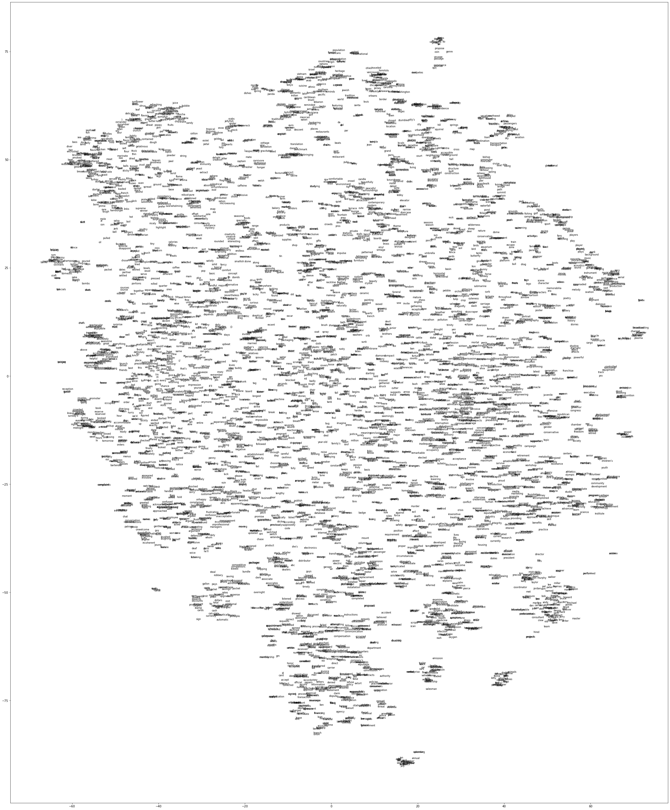
Visualization

You can begin to get a feel for what your matrix is like by poking around with vsm.neighbors to see who is close to or far from whom.
It’s very useful to complement this with the more holistic view one can get from looking at a visualization of the entire vector space.
Of course, any visualization will have to be much, much lower dimension than our actual VSM, so we need to proceed cautiously, balancing the high-level view with more fine-grained exploration.
We won’t have time this term to cover VSM visualization in detail. scikit-learn has a bunch of functions for doing this in sklearn.manifold, and the user guide for that package is detailed.
It’s also worth checking out the online TensorFlow Embedding Projector tool, which includes a fast implementation of t-SNE.
In addition, vsm.tsne_viz is a wrapper around sklearn.manifold.TSNE that handles the basic preprocessing and layout for you. t-SNE stands for t-Distributed Stochastic Neighbor Embedding, a powerful method for visualizing high-dimensional vector spaces in 2d. See also Multiple Maps t-SNE.

def tsne_viz(df, colors=None, output_filename=None, figsize=(40, 50)):
    """2d plot of `df` using t-SNE, with the points labeled by `df.index`,
    aligned with `colors` (defaults to all black).

    Parameters
    ----------
    df : pd.DataFrame
        The matrix to visualize.
    colors : list of colornames or None (default: None)
        Optional list of colors for the vocab. The color names just
        need to be interpretable by matplotlib. If they are supplied,
        they need to have the same length as `df.index`. If `colors=None`,
        then all the words are displayed in black.
    output_filename : str (default: None)
        If not None, then the output image is written to this location.
        The filename suffix determines the image type. If `None`, then
        `plt.plot()` is called, with the behavior determined by the
        environment.
    figsize : (int, int) (default: (40, 50))
        Default size of the output in display units.

    """
    # Colors:
    vocab = df.index
    if not colors:
        colors = ['black' for i in vocab]
    # Recommended reduction via PCA or similar:
    n_components = 50 if df.shape[1] >= 50 else df.shape[1]
    dimreduce = PCA(n_components=n_components)
    X = dimreduce.fit_transform(df)
    # t-SNE:
    tsne = TSNE(n_components=2, random_state=0)
    tsnemat = tsne.fit_transform(X)
    # Plot values:
    xvals = tsnemat[: , 0]
    yvals = tsnemat[: , 1]
    # Plotting:
    fig, ax = plt.subplots(nrows=1, ncols=1, figsize=figsize)
    ax.plot(xvals, yvals, marker='', linestyle='')
    # Text labels:
    for word, x, y, color in zip(vocab, xvals, yvals, colors):
        try:
            ax.annotate(word, (x, y), fontsize=8, color=color)
        except UnicodeDecodeError:  ## Python 2 won't cooperate!
            pass
    # Output:
    if output_filename:
        plt.savefig(output_filename, bbox_inches='tight')
    else:
        plt.show()

tsne_viz(yelp20_pmi)

png

[실습] VSMs(Vector-space models)